You can find all the posts on this series under the tag maps-app.

You can also find the current state of the project under my GitHub repo mapic (including the Spanish versions).

Scope of this post

When you prepare for a job interview one of the questions they always tell you to prepare is “What are you most proud of?”. Personally I’ve never been asked that question in a job interview but it kept me thinking. Some years ago I developed the R code for the creation of maps of infrastructure for a Political Sciences project, and I can say that this is one of the projects I’m most proud of. However, it is also true what they say to developers, that nobody cares about how you did it. The final user only cared about what was done, while the research team about what are the possibilities.

The project taught me so much in terms of technical skills that I have decided to share the how in case it can help somebody else. It is also my way to contribute to the R community since I myself learned R and programming thanks to the kind people who post their experience on the web (and to the ones who have the patience to answer questions in StackOverflow too). Due to the confidentiality agreement of the client, I also cannot share a git repository.

We created maps of data showing changes over a span of time for different countries and pointing at all kinds of cities. That basically means that we need to map any region of the world with R. Today there are all kinds of packages and techniques to do that. I will share the strategy I used with ggplot2 and maps packages, using support of Open Street Map to obtain the coordinates of cities and finally making it interactive with shiny.

The project itself is quite long for a single post, and just recently I managed to extract the base code I created and make it public, without compromising any privacy issues. On the other hand, it is a live project that I am currently working on. Therefore, I decided to share my path and experiences along the creation process of the Shiny app. The posts are not only about the Shiny app, but the package I created behind it. I will touch topics of functions crafting, creation of the maps, classes of objects, etc., as well as any interesting issue that appear on the way. It is my way to contribute to the R community and at the same time keeping the project documented for myself.

This first post is asbout the creation of The basic map

I hope you all enjoy it. Feel free to leave any kind of comment and/or question at the end.

Background

When I joined the team all what they knew is that the wanted to make maps of infrastructure (say hospitals, cafes, churches, public offices, etc., but the project can basically be applied to anything countable per city). The maps should change in time according to the data (usually growth) and it should be possible to apply it for any country and thus, any kind of city of that particular country can be listed there. This last point represents a challenge because to make a map you need the coordinates of a particular point to map, but instead we got address in the best scenario, or only city name in the worst. Therefore, we left it to the level of city and decided to work with that.

Most R packages to make maps have granularity up to some regions and major cities per country, and we are talking about countries where somebody has develop some R package for that. However, even the best packages would miss some cities or some countries some times. We needed to standardize everything without the need of changing packages according to the particular country. Before I joined, the team attempted to use Google Maps and excel, but the amount of data became messy and the flexibility to edit the maps was pretty limited. And they didn’t want to add copyright issues to the list of limitations. Therefore I proposed to use R. Of course, nobody in the team had ever heard about it before. We could had used any other tool, I learned that both, Python and JavaScript have some decent possibilities. But R is what I have been using for the last 10 years and is what I wanted to use for this project. And so I started to code.

The first couple of maps were custom code for a particular country with decent styles. But it quickly evolved into a set of functions and arguments to maintain the same standards for each map. The support of graphic designers also took the styles to a very professional level. After a few months we had very professional maps that could be done in couple of hrs (or less) with a couple of lines of code. Each map per each country with the desired span of years to be printed.

I don’t think I will share every single detail of it, but at least I want to show how we went from the basic map to its dynamic form mapping over a span of time, and how I wrapped it all together in a couple of functions to make it quickly replicable for any given data set. Let me know what you think.

How to create a map of any country in R using the library maps

The first step is to create the basic map of a country. Here is the function to achieve exactly that.

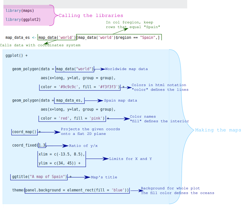
library(maps)
library(ggplot2)

## make a df with only the country to overlap
map_data_es <- map_data('world')[map_data('world')$region == "Spain",]

## The map (maps + ggplot2 )
ggplot() +
    ## First layer: worldwide map
    geom_polygon(data = map_data("world"),
                 aes(x=long, y=lat, group = group),
                 color = '#9c9c9c', fill = '#f3f3f3') +
    ## Second layer: Country map
    geom_polygon(data = map_data_es,
                 aes(x=long, y=lat, group = group),
                 color = 'red', fill = 'pink') +
    coord_map() +
    coord_fixed(1.3,
                xlim = c(-13.5, 8.5),
                ylim = c(34, 45)) +
    ggtitle("A map of Spain") +
    theme(panel.background =element_rect(fill = 'blue'))

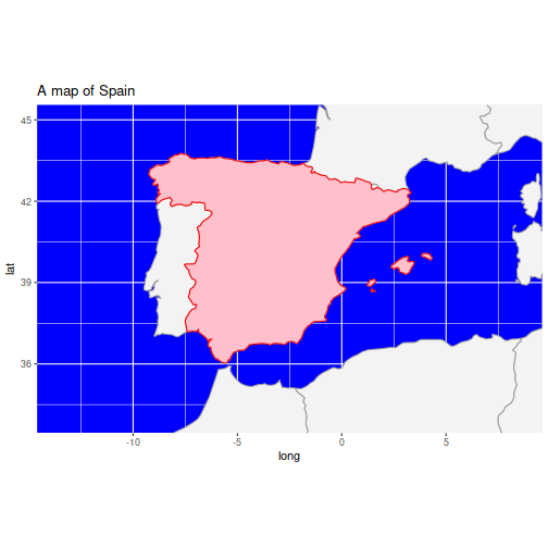
We are using the library maps in combination with ggplot2. The maps package contains coordinates system for a map of the whole world separated by countries (although political borders might not be fully up to date). It can as well do the maps, but for that we are making use of ggplot2 support here.

We start by extracting the data relevant to the country we want to map, in this case Spain. It is of course important to pass the name of the country in the same way that it is written in map_data('world')$region. You can use the function unique() to find the exact names of all the countries included in the packages (unique(map_data('world')$region) gives 252 countries at the moment of writing this post).

Once we have the data for the one particular country, we could simply map it directly using geom_polygon() however, that would map Spain surrounded by empty space around it. To place it in the context of its neighborhood, we apply two layers of geom_polygon(): first one with the map of the whole world and secondly the map of the country only.

Then we need to tell ggplot to use a coordinates system to create maps instead of just polygons. For that we use coord_map() function and then we pass the details of the map ratio, and limits in X and Y to the function coord_fixed().

Up to here we can have our map. ggplot is basically plotting what we are specifying inside the coordinates system, everything around it (the oceans) will be just empty and it will be filled in by the default grids and gray colors of ggplot(). Thus, we need to define the color of the Oceans as the background color for the whole plot. That’s what the last line of code does.

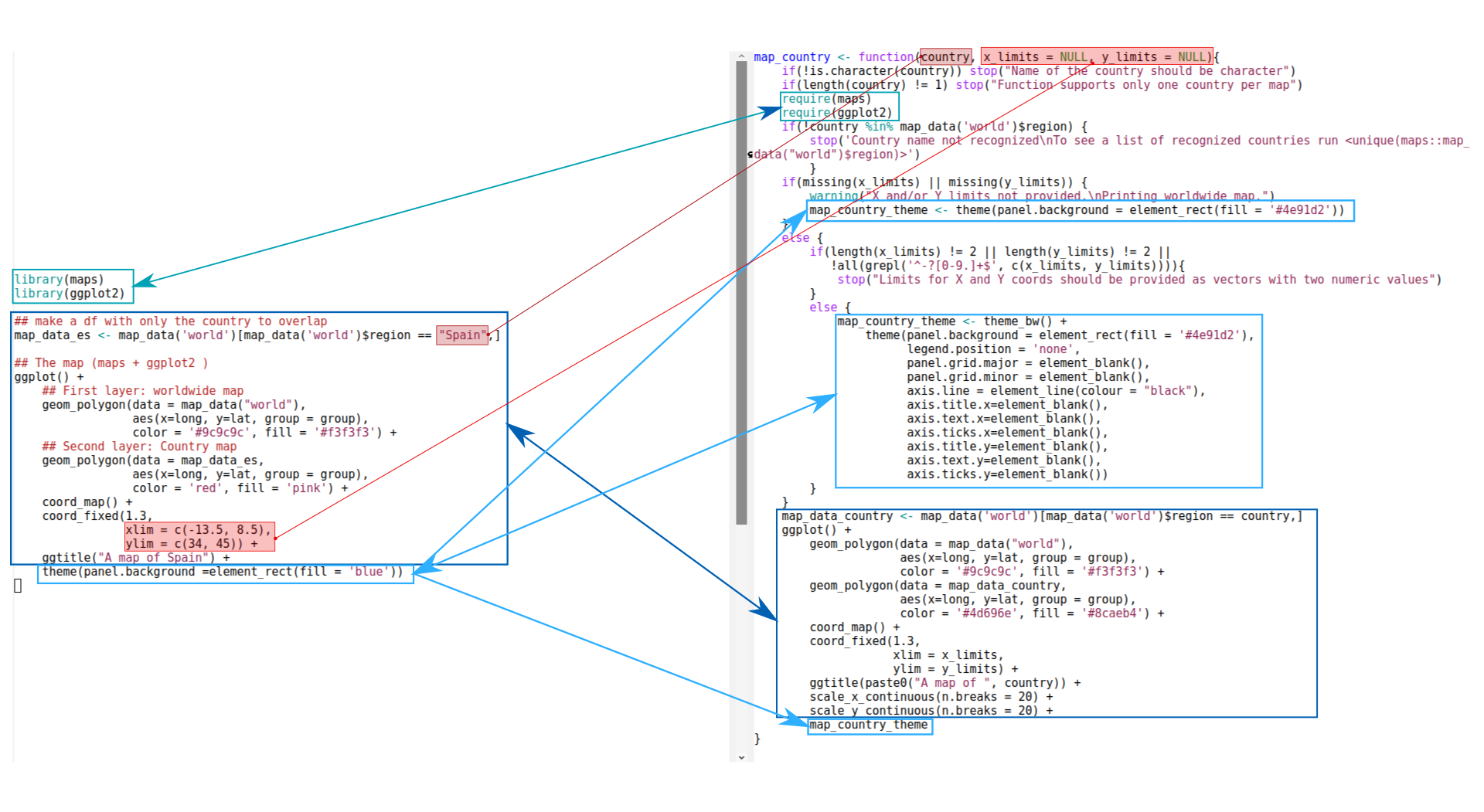
Of course there are a lot of improvements to do. So far I have given exaggerated colors to make obvious for the reader which piece of code controls what. In that sense you can see that you can simply pass the names of the colors, which applies the defaults, or you can be more specific and provide the html notation of the color (i.e., '#9c9c9c'). So, let’s now improve the visuals and at the same time create a function to plot any country we want to.

Function to create the basic map in R

map_country <- function(country, x_limits = NULL, y_limits = NULL){
    ## Verifying the arguments passed to the function
    if(!is.character(country)) stop("Name of the country should be character")
    if(length(country) != 1) stop("Function supports only one country per map")
    ## Load libraries
    require(maps)
    require(ggplot2)
    if(!country %in% map_data('world')$region) stop('Country name not recognized\nTo see a list of recognized countries run <unique(maps::map_data("world")$region)>')
    ## If coords limits missing, print worldwide map with coordinates system to allow
    ## User observe coords for reference
    if(missing(x_limits) || missing(y_limits)) {
        warning("X and/or Y limits not provided.\nPrinting worldwide map.")
        map_country_theme <- theme(panel.background = element_rect(fill = '#4e91d2'))
    }
    else {
        if(length(x_limits) != 2 || length(y_limits) != 2 ||
           !all(grepl('^-?[0-9.]+$', c(x_limits, y_limits)))){
            stop("Limits for X and Y coords should be provided as vectors with two numeric values")
        }
        else {
            ## All the received inputs are correct.
            ## Let's define our custom theme for the final map 
            map_country_theme <- theme_bw() +
                theme(panel.background = element_rect(fill = '#4e91d2'),
                      legend.position = 'none',
                      panel.grid.major = element_blank(),
                      panel.grid.minor = element_blank(),
                      axis.line = element_line(colour = "black"),
                      axis.title.x=element_blank(),
                      axis.text.x=element_blank(),
                      axis.ticks.x=element_blank(),
                      axis.title.y=element_blank(),
                      axis.text.y=element_blank(),
                      axis.ticks.y=element_blank())
        }
    }
    ## make a df with only the country to overlap
    map_data_country <- map_data('world')[map_data('world')$region == country,]
    ## The map (maps + ggplot2 )
    ggplot() +
        ## First layer: worldwide map
        geom_polygon(data = map_data("world"),
                     aes(x=long, y=lat, group = group),
                     color = '#9c9c9c', fill = '#f3f3f3') +
        ## Second layer: Country map
        geom_polygon(data = map_data_country,
                     aes(x=long, y=lat, group = group),
                     color = '#4d696e', fill = '#8caeb4') +
        coord_map() +
        coord_fixed(1.3,
                    xlim = x_limits,
                    ylim = y_limits) +
        ggtitle(paste0("A map of ", country)) +
        scale_x_continuous(n.breaks = 20) +
        scale_y_continuous(n.breaks = 20) +
        map_country_theme
}

## Test the function with a different country
map_country("Germany", c(-2, 22), c(47, 55))

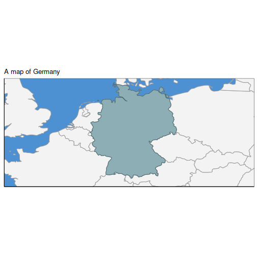
Although the function might seem complicated at first, it is in fact the same code as we used to create the map, but instead of typing directly the name of the country or the limits for X and Y, we replace them with the arguments country, x_limits and y_limits respectively; in that way all the parts were we had the string "Spain" we now have the argument country, and so on. These are the only arguments that we need to change when we want to map a different country. You can define more arguments in case you want to have more possibilities to be editable, for example, we could define an argument country_color to specify the color we want for the target country. In our case we wanted to keep the same standards for all the maps due to branding reasons and thus, we rather wanted to have the exact same colors and styles for all of our maps.

There are also some additions on the top before the actual code to make the maps, all the if and else statements that are simply used to validate that the information passed by the user is the info that we actually need to make the function work. If any incorrect argument is passed to the function, we stop the process and write a message of what is wrong using the function stop(). For the case that no limits of either X or Y are defined, I send a warning message using warning(). In that case the process continues but we define a theme() that allows the user to see the country in the context of the worldwide map, with excess of values in the X and Y axes to provide the points of reference and give an idea of where to set the limits. By the end, when we ensure that all the values are fine, we define the final theme that we actually want to apply. About that, probably I should make special mention of !all(grepl('^-?[0-9.]+$', c(x_limits, y_limits)))): it is used to ensure that X and Y limits are of type numeric. See the visualization of the code below together with the help of the function(s) you don’t understand for a more detail explanation. Feel free to test the errors and warnings by providing to the function no country names or letters where there should be numbers, etc.

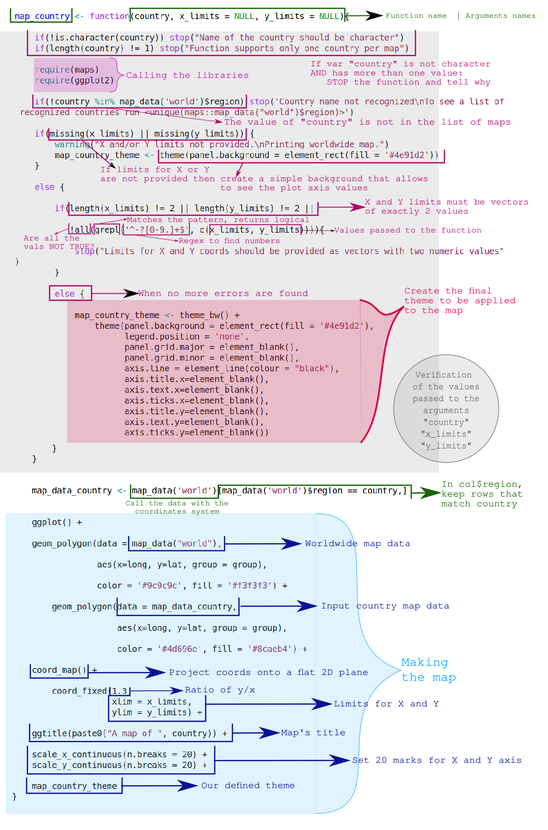
The lower part of the function is exactly the same as our first map, replacing the actual values for the arguments. We also have changed the colors for more specific ones. Almost by the end of the function we have added scale_x_continuous(n.breaks = 20) which will add 20 marks of the X axis scale (same for Y). We want to use it to ensure that, in case the user doesn’t have idea of which limit values to choose, it can have a good approach regarding the position of the target country. In case that both limits for X and Y are passed to the function, our other theme will mask this 20 breaks with axis.text.x = element_blank() and axis.ticks.x = element_blank().

The final line is the test that our function can plot a map other than Spain, in this case I chose Germany. We can basically choose any country included in the maps package and now make the map with the same standards in one line of R code.

Final remarks

Here I am somehow showing one of the methods I use to create functions: I basically write first the code of what I want to achieve and once it does exactly what I want, I wrap it in a function, replacing the arguments that the user will need to modify later. Then I think what could go wrong and create the corresponding warnings an errors. It is a good practice to do that not only for the user to know better how to use the function, but also for yourself, it proves very useful when we need to debug code. Another good practice in R functions is the call to the libraries inside the function using require(). Even if you are writing many functions that use the same libraries, is good to repeat it on each function, or per script, to make it self contained and again, help yourself in the debugging process. Not long ago I started collaborating in a project where there was no call to the libraries per function, but rather only at the top level when the main action of the program was called. This made almost impossible for me to test and debug code so, the first activity I did as a new member of the team was to spend 2 full working days adding require() where necessary.

I hope you get some fun mapping different countries. Because different countries have different sizes and shapes, one way to improve the visuals related to this is by adjusting the ratio, for example, my own map of Germany looks out of shape, but it improves considerably if instead of 1.3 we give a ratio of 1.4, check the documentation to learn more about it.

Once that we have the basic map, we could add the cities were we want to add data values. Unfortunately, for cities there are many limitations, specially for countries where no special packages has been created to be mapped, and even there, most packages of particular countries don’t contain all the cities, especially minor ones. Thus, in our second part I will show how I tackled this problem doing some web scrapping to open street maps.